Project notes
Bitcoin vs SPY: returns, risk and the cost of timing
A Python analysis of Bitcoin and US equities, exploring how drawdowns, investment timing and the choice of starting date change the story behind headline returns.
- Python
- pandas
- NumPy
- Matplotlib
- Jupyter
Bitcoin’s historical growth makes for a striking chart. But an ending balance says little about the losses along the way, or what happened to someone who started investing years later.
For this project, I compared Bitcoin (BTC) with SPY, an exchange-traded fund tracking the S&P 500. I built a sequence of Python notebooks covering growth, monthly returns, volatility, risk-adjusted performance, correlation and investment strategies. The final step was to move the starting date and see which conclusions survived.
The main finding: BTC delivered much greater compounded growth over the full sample, alongside much greater risk. Its advantage narrowed sharply on a risk-adjusted basis, and some later entry dates reversed the ranking against SPY.
This write-up uses the project’s saved data snapshot: 27 December 2013–12 November 2026, with all amounts in nominal US dollars. The results describe that snapshot; the underlying provider data was not independently audited during compilation.
Building a comparable dataset
The acquisition notebooks use Alpha Vantage for BTC/USD and yfinance for SPY, with automatic price adjustment enabled. I filtered BTC to positive-volume observations, selected closing prices and joined the two series on shared dates. That produced 3,239 prices and 3,238 paired returns, spanning approximately 12.88 years.
SPY’s adjusted prices serve as a dividend-reinvestment proxy. BTC uses its closing price. This makes the comparison closer to an investment-return comparison than a comparison of unadjusted price charts.
The shared calendar is an important compromise. Bitcoin trades on weekends; SPY does not. Calculating returns after joining the dates means BTC’s next shared-date return includes the intervening price movement. Matching date labels also does not guarantee identical provider closing times. The results therefore describe this aligned dataset, including its limitations.
The workflow uses pandas for alignment and aggregation, NumPy for numerical calculations, and Matplotlib for charts. Ten notebooks take the project from acquisition to start-date sensitivity. A report compiler checks core calculations against the saved exports and packages the results with machine-readable tables.
The headline return hides the journey
With $100 invested at the beginning and no further contributions, BTC ended at $10,013.70, compared with $510.92 for SPY.
| Full-period metric | BTC | SPY |
|---|---|---|
| Ending value of $100 | $10,013.70 | $510.92 |
| Total return | 9,913.70% | 410.92% |
| Compound annual growth rate | 43.01% | 13.50% |
| Annualised volatility | 66.25% | 17.13% |
| Maximum drawdown | −82.90% | −33.72% |
Download the underlying metrics (CSV).
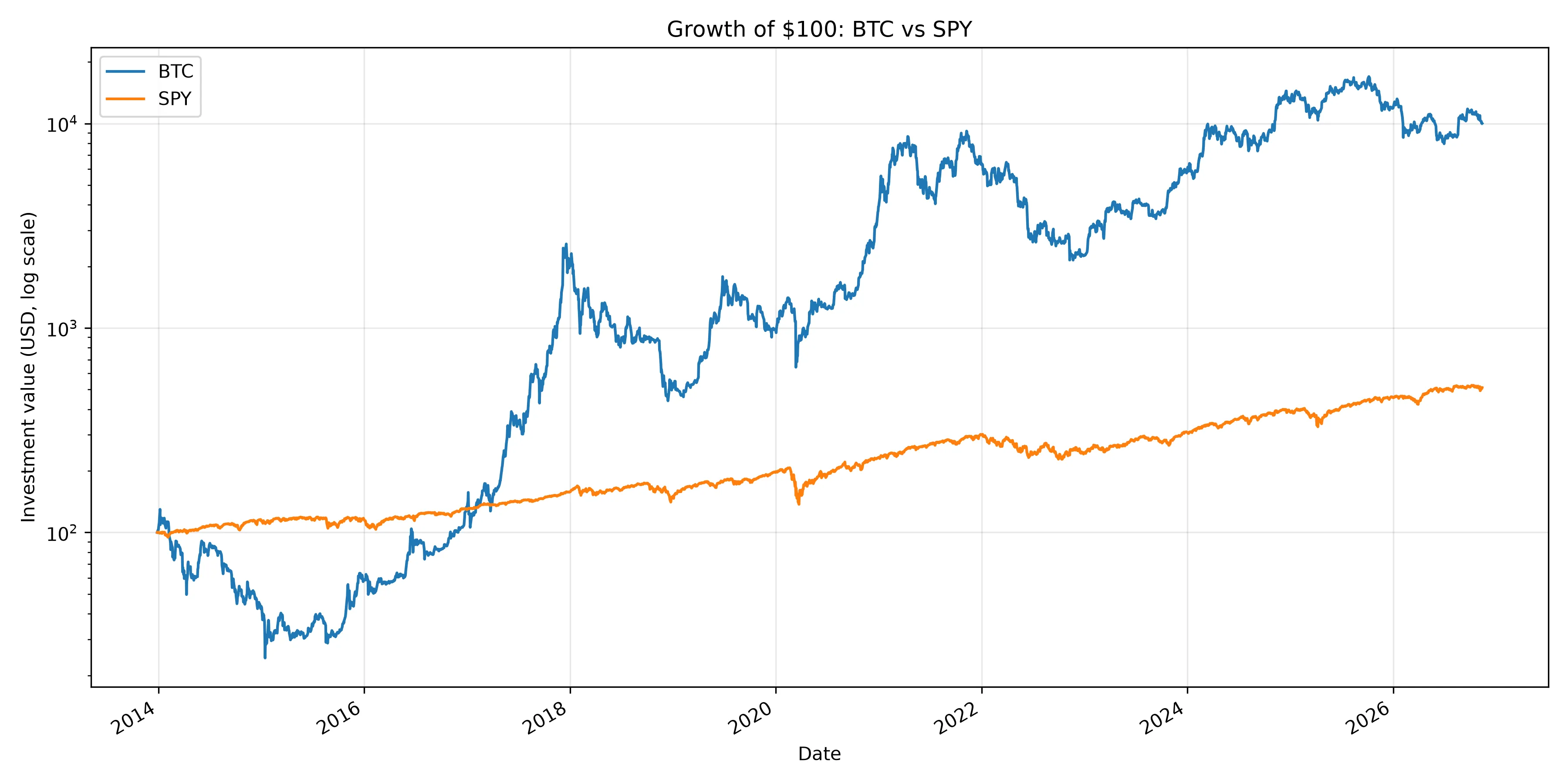
Growth of $100 on a logarithmic scale. Equal vertical distances represent equal multiplicative changes, so both growth paths remain visible.
Compound annual growth rate (CAGR) expresses the start-to-finish change as an equivalent constant annual rate. It is not the return earned in a typical year. Here it uses actual elapsed days divided by 365.25.
The path was much less smooth than the CAGR suggests. BTC’s annualised volatility was approximately 3.87 times SPY’s. Both estimates use the sample standard deviation of aligned returns multiplied by the square root of 252; using 365 for BTC alone would mix conventions on the same shared calendar.
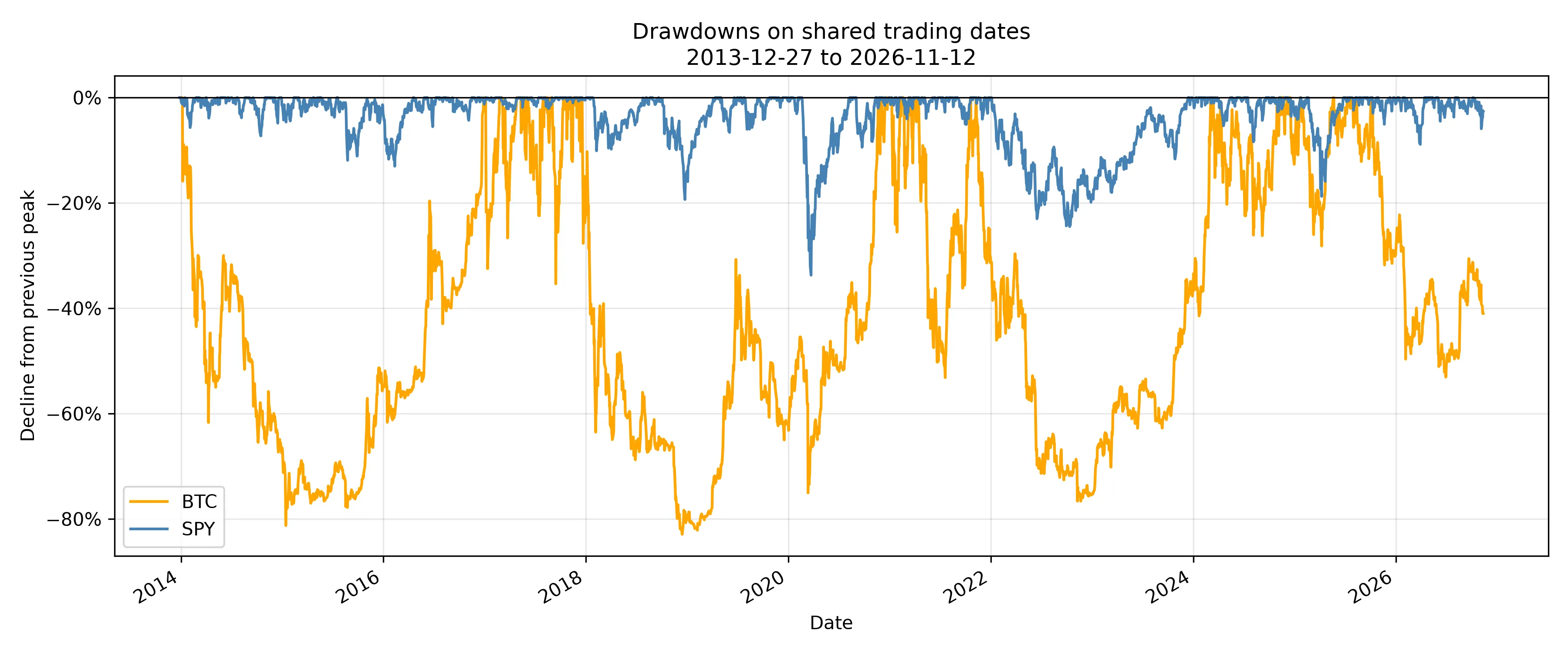
Drawdown measures the loss from the highest value reached so far. These observations use shared-date closes and exclude intraday and unobserved weekend extremes.
Monthly results show another distinction. Across 154 complete months, January 2014–October 2026, SPY gained in 68.18% of months, versus 54.55% for BTC. Yet BTC’s average monthly return was 5.10%, compared with SPY’s 1.15%. Larger gains and more frequent gains are different properties. November 2026 is incomplete and excluded from these statistics; any 2026 annual figure is year-to-date through 12 November.
Adjusting for risk changes the comparison
To put return alongside risk, I calculated three ratios. Sharpe compares mean excess return with volatility; Sortino uses downside deviation relative to a target return; Calmar divides CAGR by the magnitude of maximum drawdown.
| Ratio | BTC | SPY |
|---|---|---|
| Sharpe | 0.875 | 0.827 |
| Sortino | 1.307 | 1.165 |
| Calmar, full sample | 0.519 | 0.401 |
BTC’s Sharpe ratio was only slightly higher, despite the enormous gap in ending wealth. That is a more qualified result than the growth chart alone suggests.
These calculations use 0% for both the risk-free rate and the Sortino target, rather than historical cash yields. Sortino’s downside deviation includes all observations, assigning zero downside to returns above the target. Calmar uses the full sample rather than a trailing three-year window. No confidence intervals or significance tests were calculated, so the ratios do not establish statistical superiority.
Correlation changes through time
The full-period Pearson correlation of paired returns was 0.222. A single number, however, hides changes in how the two assets moved together.
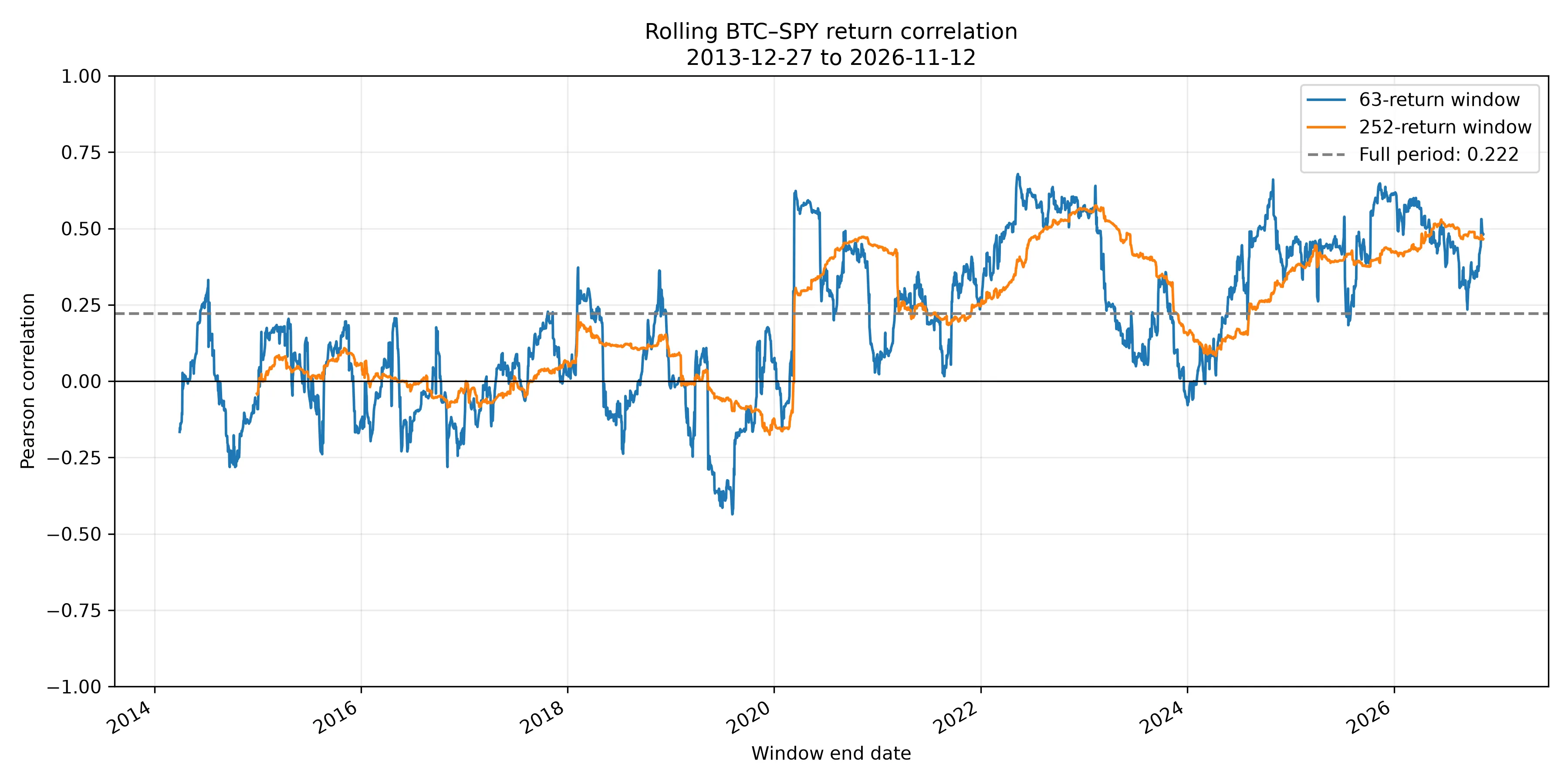
Rolling correlations over 63 and 252 paired returns. The dashed line marks the full-period correlation.
The shorter window ranged from approximately −0.436 to +0.678. At the final observation, the 63-return correlation was 0.481 and the 252-return correlation was 0.465, both above the full-period value.
This is evidence of a changing relationship, not proof that BTC protects against equity losses. A dedicated analysis of periods when SPY falls would be needed to test that claim. The rolling windows also overlap, so their estimates are not independent observations.
Investing immediately or spreading purchases out
I next compared two ways of deploying the same $12,000 available upfront. One invests everything immediately. The other splits the budget across 156 monthly purchases of approximately $76.92, from the initial observation to November 2026.
Purchases use the first shared observation of each month. Fractional units are allowed, idle cash earns zero, and fees, spreads and taxes are excluded. Account value includes both investments and unspent cash.
| Asset and strategy | Ending wealth | Account CAGR | Max drawdown |
|---|---|---|---|
| BTC · lump sum | $1,201,644.58 | 43.01% | −82.90% |
| BTC · monthly | $599,190.04 | 35.49% | −78.78% |
| SPY · lump sum | $61,309.96 | 13.50% | −33.72% |
| SPY · monthly | $33,075.19 | 8.19% | −20.10% |
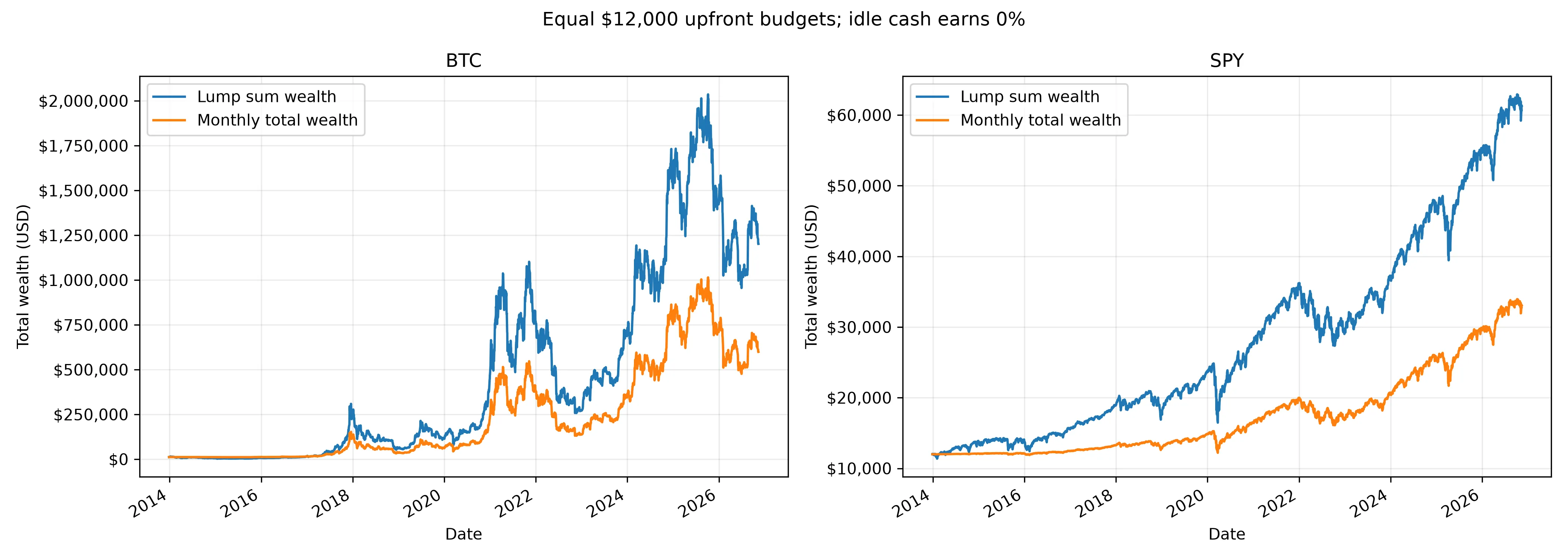
Each strategy starts with its own $12,000 budget. Wealth includes idle cash; the two asset panels use different dollar ranges.
Lump sum produced more ending wealth for both assets in this example. Monthly deployment reduced the observed maximum account drawdown, but kept part of the budget out of the market for years.
Cash accounting matters here. BTC’s monthly strategy had an invested-sleeve XIRR of 54.47%, which measures the money-weighted return on the dated purchases. Its whole-account CAGR was 35.49%, which includes the cash waiting to be invested. The higher XIRR does not mean it made better use of the original budget.
This experiment concerns capital already available at the start. It does not compare investing salary as it arrives with an earlier lump sum that the investor never had.
To reduce reliance on one entry date, I repeated the comparison over one-, three- and five-year horizons, using 12, 36 and 60 monthly purchases respectively. Lump sum finished ahead in 85.42% of BTC’s 96 five-year scenarios and all 96 SPY five-year scenarios. These overlapping historical windows are not independent trials or forecasts of future win probabilities. Assuming zero cash interest also affects the comparison.
What if we remove the early Bitcoin years?
The final experiment moves the starting date while keeping 12 November 2026 as the endpoint. It covers 144 monthly starts with at least one year remaining, producing 576 combinations of start date, asset and strategy. Every account begins again with $12,000.
| Starting date | BTC lump sum | SPY lump sum |
|---|---|---|
| 27 December 2013 | $1,201,644.58 | $61,309.96 |
| 2 January 2018 | $59,129.90 | $38,703.44 |
| 3 January 2022 | $19,026.50 | $20,317.06 |
| 2 January 2024 | $19,647.23 | $19,904.22 |
| 2 January 2025 | $9,115.21 | $15,887.70 |
Ending wealth from the same $12,000 starting budget, valued at the common endpoint. Later entries have shorter holding periods.
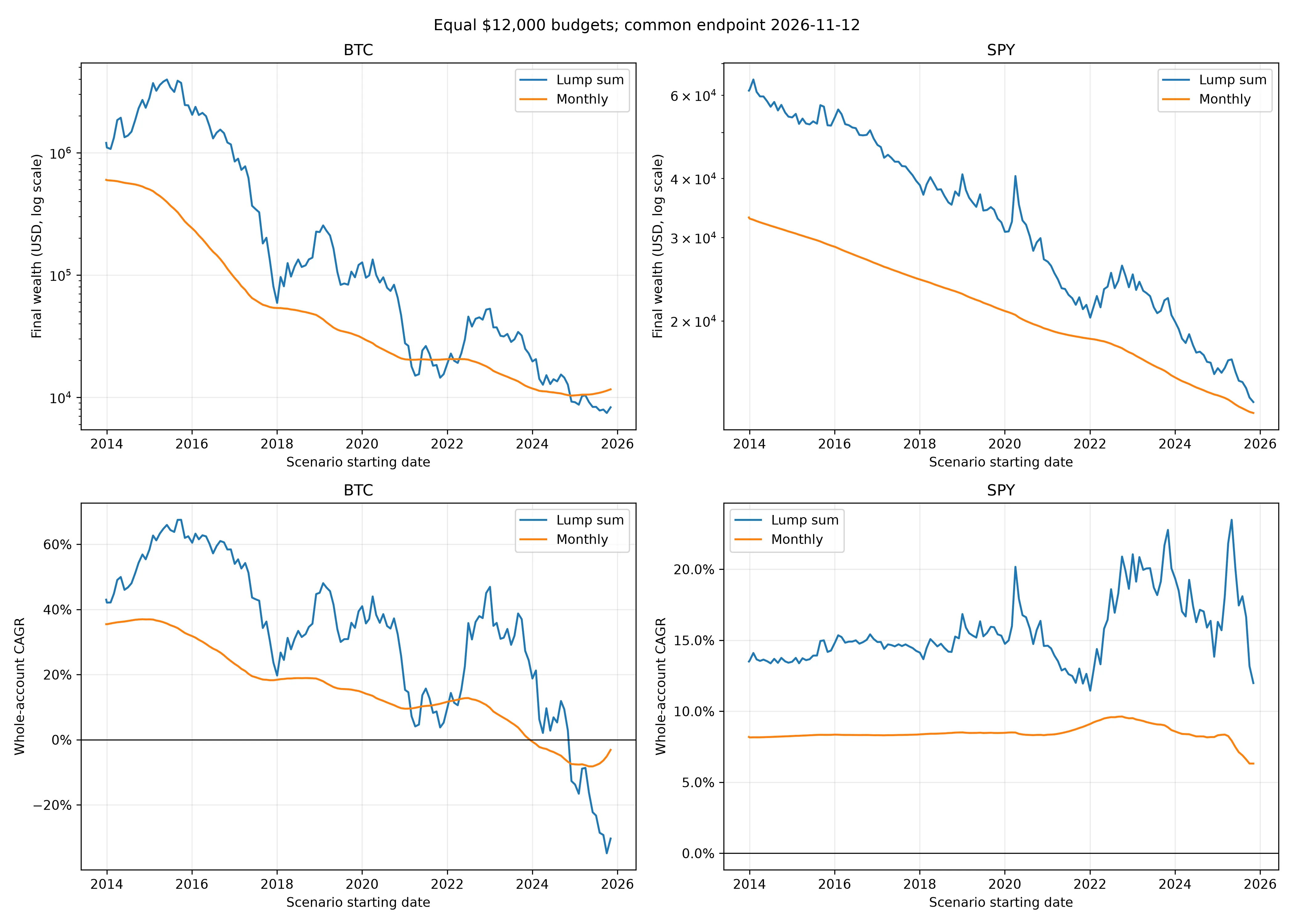
The horizontal axis is the entry date of a new hypothetical account, not the passage of time for one portfolio.
Starting in January 2018, BTC still finished ahead. Starting in January 2022, SPY slightly beat BTC for lump-sum investing, while BTC finished ahead for monthly deployment. Starting in January 2025, both BTC strategies ended below their initial budgets, while both SPY strategies ended above them.
These examples demonstrate sensitivity to entry date. They do not establish that later Bitcoin investment always underperformed. Keeping the endpoint fixed also entangles timing with holding duration; annualising returns does not make the market conditions equivalent. That is why this experiment complements the fixed-horizon comparisons rather than replacing them.
What I took from the project
The most useful part of this analysis was making the comparison rules explicit. Aligning dates changes what a daily return represents. Including idle cash changes the meaning of strategy performance. Moving the starting date changes which investor experience the headline result describes.
Within this snapshot, BTC’s larger compounded return came with much deeper losses and a smaller advantage on the chosen risk-adjusted measures. SPY had a higher frequency of positive months. Neither a low average correlation nor a favourable full-period return answered every question about risk or investment timing.
The next extensions I would prioritise are historical cash yields, synchronised closing times, and a fixed 12-month deployment schedule followed by several holding periods. Recovery times, performance during equity losses and uncertainty estimates that account for time dependence would add context that this project does not yet provide.
Data and reproducibility
The analysis is historical and descriptive. It excludes inflation, trading costs and taxes. The BTC volume filter, the common starting date and provider adjustments affect the results. The compiler independently recalculated core metrics from the saved aligned prices; this checks internal consistency, not the accuracy of the providers’ original market data.
Selected exports used in this write-up are available below. Return, volatility and drawdown fields in the core metrics are decimals: 0.4301 represents approximately 43.01%. Strategy return, growth, drawdown, win-rate and relative-advantage fields also use decimals. The monthly performance export instead stores percentages. Risk-adjusted ratios and correlations are unitless; prices, budgets and wealth are in USD.